Figure 1. Compute Engine Panel
Compute Engine Panel
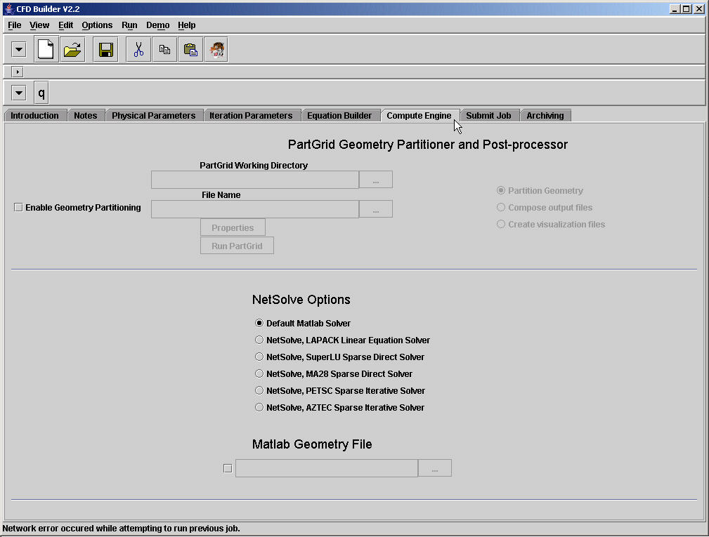
The original goal of the GUI was to provide a generic tool for solving computational simulation examples. The reality of any useful simulation is that there always be some compute engine specific tools. These tools were separated from the rest of the GUI and placed in the Compute Engine Panel.
Figure 1. Compute Engine Panel
At the top is the PartGrid Geometry Partitioner. This is parallel pre- and post-processor used with the PICMSS compute engine. Below the divider are Matlab specific options for NetSolve and Matlab geometry formatted files.
PartGrid Geometry Partitioner
The primary goal of the PartGrid Geometry Partitioner is to divide a Patran formatted neutral file geometry into several parts.
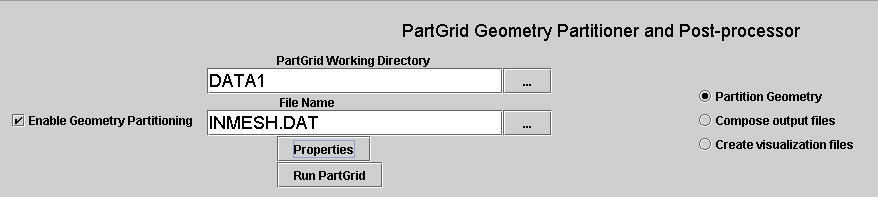
Figure 2. Partitioning a geometry in a Patran neutral file.
To run PartGrid,
1. the panel must be activated by selecting the checkbox to
the left.
2. The geometry partitioning option must be selected on the right.
3. When Partgrid runs it will generated several files. Specify the location
of these files in the Working Directory.
4. Specify the Patran neutral file name, which should include path information.
Use the File Choosers for both of these options. More information of the
File Chooser can be found in the Additional Tools section of the Help Topics.
5. PartGrid requires information about how the grid is to be partitioned.
This information includes initial condition data, which must be partitioned
as well. This information can be refreshed from the default (2-D), opened
from, or saved to, a file.
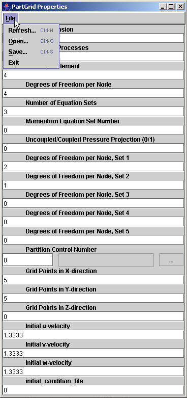
Figure 3. Partgrid options.
a. Dimension of the mesh (1,2, or 3)
b. Number of processes (number of partitions)
c. Number of elements per node.
d. Degrees of freedom per node
e. Number of equation sets.
f. Which set is the momentum equation set.
g. Is stability mechanism coupled with momentum (0/1 , no/yes)
h-l. How many degrees of freedom per set.
m. Use METIS grid partitioning algorithm (0), or specify partitioning with a file (1)
n-p. How many grids points occur in x, y, and z (benign).
q-s. Specifiy initial condition on inlet in x, y, and z.
r. Specify the type of initial condition (0/1/2, slug/file(INICON.DAT)/parabolic)
After PICMSS has run, the output files containing data for each process may be composed into a single file with a user provided filename. This file may be used as an initial condition to the compute engine, specified as a restart file in the Submit Panel.
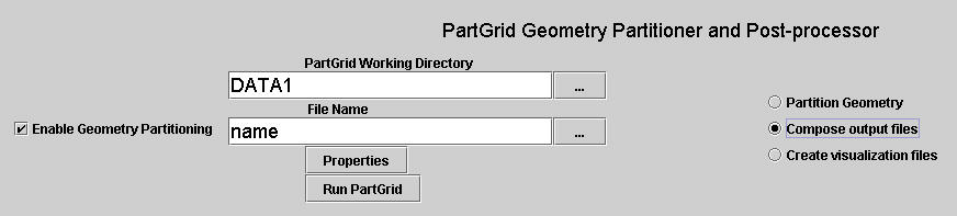
Figure 4. Composing the output files.
An output file may used to generate visualization formatted files from a composed output file. In this case, Tecplot and VTK formatted files are generated.
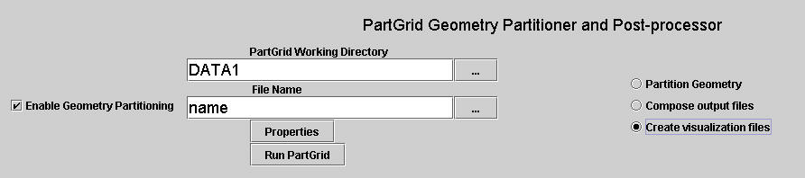
Figure 5. Generating visualization files.
NetSolve Options
NetSolve parameters are defined by the programming language chosen by the user. For Matlab, any NetSolve option chosen will put Matlab formatted script into the template for running NetSolve problems. This option requires that the user have a NetSolve client. If running remotely, this option is provided to the user. If running Matlab locally, the user must download and install the Matlab client.
Matlab Geometry File
One of the more complicated aspects of computational simulation is geometry generation and specification. For 1-D problems this is simple as a 1-D domain is only a line. Matlab provides the ability to specify a line quite simply, so no geometry file is required for 1-D problems. When the dimension increases to 2-D (3-D options not yet available) then a file must be specified in a particular format including boundary locations and names.
X1 X2 121 2
0.000000 10.000000
0.000000 9.000000
0.000000 8.000000
0.000000 7.000000
....
elcon 100 4
2 13 12 1
3 14 13 2
4 15 14 3
5 16 15 4
....
XL 11
1 2 3 4 5 6 7 8 9 10 11
XR 11
111 112 113 114 115 116 117 118 119 120 121
YT 11
1 12 23 34 45 56 67 78 89 100 111
YB 11
11 22 33 44 55 66 77 88 99 110 121
...
Three pieces of information are required in the Matlab formatted geometry file.
1. The location of each node. In the header the names X1 and
X2 are expected with the number of nodes and the number of dimensions. The
order of the nodes is expected to be from 1 to N.
2. The element connectivity. The elcon header name is expected with the
number of elements and the number of nodes per element. The element number
follows the ordering of the nodes in the previous section, so the must not
be a node number greater than N.
3. The location of the boundary must be specified. In the header, the name
of the boundary is supplied with the number of nodes on that boundary. In
order for these nodes to take a boundary value, the names must correspond
to the names supplied in the Boundary Conditions window, discussed in the
Equations Panel.