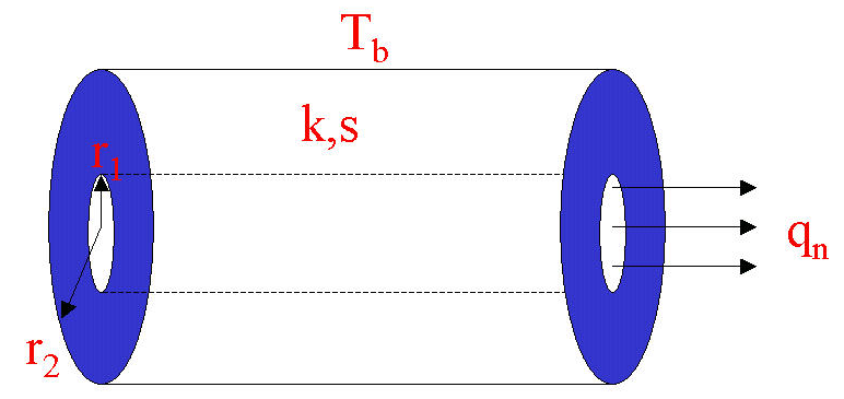
Figure 1. Axisymmetric pipe with source.
Tutorial
This tutorial is separated into 2 parts. The first tutorial is the easiest, allowing the user to get comfortable with the graphical user interface before actually building equations. The second tutorial is more comprehensive, guiding the user through building equations, Jacobians, and boundary conditions, then executing the simulation. In each tutorial the same model will be used so that similarites are more apparent to the learner. Several pictures were included with the documentation for clarity so they may take a few moments to load.
Problem description:
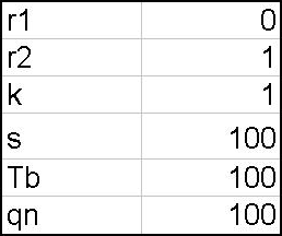
Consider a fluid flowing through a thick axisymmetric pipe. The fluid is heated with known constant properties such that the pipe inner surface temperature and heat convection coefficient are known. Thus the flux boundary condition (qn) on the inner surface is a known constant. The outer surface temperature (Tb) is held constant, and the pipe material properties (k) are known (see Figure 1). A known constant source (s) is applied to the interior of the domain. The desired solution is an accurate (0.1oF) estimate of the inner surface temperature. Because of axisymmetry, the energy equation solution is calculated as a 1-dimensional problem from r1 to r2..
Figure 1. Axisymmetric pipe with source.
Tutorial 1 - A Simple Demonstration
Tutorial 2 - Making Changes to a Simulation
Tutorial 3 - Creating a Simulation