Tutorial 3

The purpose of this tutorial is to take the user through the steps of building a simulation from scratch. Tutorials 1 and 2 should be completed before continuing with Tutorial 3. If the GUI is still open from those examples, go to the Menu Bar and press "File -> New". Notice that this example is specific to the Matlab compute engine.

The design philosophy of the GUI attempts to present the parts of a computational simulation in logical categories. To complete a successful simulation, each of these categories must be filled in correctly. The GUI presents an environment for the user to enter simulation information with very few restrictions. By design, the GUI understands little about computational mechanics so that users are not restricted by a limited set of rules for developing equations and parameters. Thus, it falls to the user to ensure that the simulation data is correct.

The categories to be satisfied are:

1. Data ("Constants") definition - this includes Physical, Iteration, and Integration Parameters.
2. Variable definition - define the dependent variables of the system of equations
3. *Initial conditions - every variable must have an initial condition associated with it.
4. Build equations - define equations for all sets
5. **Build Jacobians - each set of equations must have a Jacobian set associated with it.
6. Boundary conditions - for well-posedness, each equation must have boundary conditions associated with it.NOTE: The GUI will not throw an error if no boundary conditions are supplied, but the compute may not produce reasonable results..

It is recommended that the user follow these steps in this order, or at least a consistent order, every time a simulation is to be built or debugged. As the simulation grows, the amount of information can become confusing, and this process presents a logical set of steps that can be followed to cover each area of concern.

* Linear and steady equations don't typically need initial conditions, but since all equations are solved as non-linear (see **) then every variable must have a place to get started.
** For most compute engine interfaces (i.e. Matlab), all equations are treated as non-linear, even if they are linear. This was done for generality as linear equations are a special case of non-linear equations.

1. Data definition

a. Navigate to the Physical Parameters panel.
b. Enter the following information in the Dimensional Parameters table (we will not use the Non-Dimensional Parameters table here).

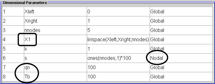
Figure 1a. Data Definition

Comments:

1) Data entered into this table does not have to used in the equations. Notice, for example, that Xleft, Xright, and nnodes will not be used in the equations, but instead are used to help define X1.
2) The variable name X1 describing the domain is required in this table, if a file is not specified describing the domain. In this case, a file will not be specified.
3) Notice that X1's value is a Matlab function. The third column is "lilteral". That is, Matlab script may be used to define a variable name. This line will show up in the Matlab script as "X1=linspace(Xleft,Xright,nnodes);"
4) The variable s is defined as nodal data. It takes the same value on every node in the domain, but it couls easily be redefined do vary with X1.
5) The variables qn and Tb are boundary condition data and will be used later. Often, the user may not know all the data that is required in the begininning, so several trips back to this table will be necessary.
6) If there are not enough rows to enter data in, enter the text box at the bottom of the table next to the label "Add more rows", enter a value for the number of rows to add, and press the Add button. In this example, 3 more rows will be required. Extra, unused rows are allowed.
7) Notice the button pad to the left of the table. As constant names are defined, those names appear on the button pad.

Figure 1b. Placing components on the Variable Toolbar for builgin equations.

c. The variables k and s will be used, later, to build equations. To the left of the Dimensional table, on the button pad, press the buttons for k and s, one time each. Notice that the buttons appear in the Variable Toolbar at the top.

d. This is a linear and steady state equation system, so no data definition is required in the Iterations Panel.

2. Variable definition

Several automated functions are provided to aid the user in build the information of a computational simulation. The GUI must be told about the equation system dependent variables.

a. Navigate to the Equation Builder panel.
b. In the first box, enter the variable name q. In our equation system we have one variable for which we will calculate a solution. It is a scalar variable representing the temperature on every node in the domain. The variable name T could have as easily been used, but for consistency with the remaining tutorial, enter q.

Figure 2. Defining the dependent variables.

Comments:

1) The user may define as many variables as the choose, whether those variables are used or not.
2) Care must be taken when choosing variable names. The GUI analyses equations based on the variable names. If the variables a, b, and ab are all defined, if the GUI encounters a variable ab, it will not know if this is a, and b, or ab (as a person will would not know). The GUI will pick one option, move on, and will not throw an error.
3) To enter another variable, click in the empty box, or tab to the next box, and a new, empty box will appear. Try not to create too many empty boxes.
4) Notice that as each variable is entered by the user, the variable will appear in the Variable Toobar. This can be used to creating equations.
5) Greek symbols can be used by pressing the last icon on the Control Toolbar. This open a window of Greek symbols. Enter the text box to place the Greek letter in, then press the Greek symbol button of choice.

3. Initial Conditions

Before continuing in the Equation Builder, and since we are in the mind-set of the dependent variables, we can go ahead and define the initial condition for each variable.

a. In the Menu Bar, press Options -> Initial Conditions

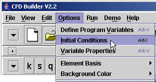
Figure 3. Open the Initial Condition window.

b. By default, the initial condition is defined as the variable name with a zero on the end. Remove the variable name and leave only the zero so that the initial condition is defined as a constant of zero over the entire domain.

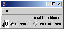
Figure 4. Initial condition for variable q, value, and type.

Comments:

There are several ways to define the initial condition.

1) A constant value (a real number) can be applied over the entire domain, as shown above (it does not have to be zero).
2) A variable can be supplied (as imlplied by the default variable q0) which is constant over the domain. This variable must be a global constant (scalar).
3) If a non-constant function is to be used (as one might be used in the Physical Parameters table) that function may be supplied directly in the Initial Conditions value text box. The radio button for "User Defined" should then be activated. Remember that if the user defines the initial condition, it is the user's responsibility to ensure that it is defined for every node in the domain.

4. Build Equations

a. For this example there will one equation set. In the Equation Builder panel, enter the text box next to the questions "How many sets do you want to build?" Enter 1, and press the Ok button.

Figure 5. Define the number of equation sets.

b. To activate an equation box, enter the inactive equation box. Notice that as an equation box is activated, a new, inactive equation box appears. The user can enter as many equations as desired. NOTE: Only activate the number of equation boxes required. Extra, empty, equation boxes may cause problems.
c. Use the Variable and Operator Toolbar at the top to build the following equation. The Operator Toolbar may need to be expanded to view the predefined operators (press the arrow to the left of the bar to expand and collapse). The keyboard may also be used for entering English letters

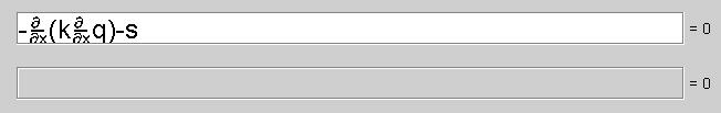
Figure 6. Entering the energy equation term with a source.

Comments:

1) Building equations requires knowledge of the end product. Matrix equations must be consistent in dimension, and this must be reflected in the above equation. This is donw by the definition of the source term as "nodal" in the Physical Parameters.
2) There are rules that must be applied to building equations in the GUI. For more information see the Help Topic Equation Building Rules.

7. Build Jacobians

By default, the Jacobians are not show so that more room is available for the user to view equation sets.

a. Next to the label "Jacobian Set Number 1", press the Show button. An empty (with zero) Jacobian box will appear.
b. An automated Jacobian building function is available for simplistic equations, but parameters must first be defined. Press the Properties button.
c. For a description of the different Jacobian Properties, see the Equation Builder Help Topic. Enter the following information: (after the Number of Equations and Variables is entered into the text box, remember to press the Define Variables button)

Figure 7. Jacobian Properties.

d. Close the Window by pressing the X in the upper right-hand corner of the Jacobian Properties window.
e. In the Equation Builder panel press the Build Jacobians button. The result should appear as Figure 8. NOTE: The Jacobian Builder is not a comprehensive Jacobian generator. It is meant as a starting point for the user. It is the user's responsibility to ensure that the Jacobians are correct.

Figure 8. Lab 2 Jacobians

6. Boundary Conditions

Every equation must have boundary conditions associated with it for well-posedness. As equations are built for each set, it is a good idea to go ahead supply the boundary condition information for each equation.

a. Open the boundary condition window for a single equation by pressing the BCs button next to the equation.(In this case we have only 1 equation)
b. There will/may be a boundary condition for every boundary in the domain. This example has a 1-D domain, which is a line. There are 2 boundaries in this domain: a point on the left end, and a point on the right end. Thus, there will be 2 entries in this BC window, one for each boundary.
c. Each boundary has four pieces of information associated with it:

1) Boundary Name - The compute engine must have a way to identify a boundary. This identification is done by giving each boundary a name.
2) Equation - This is the value that the boundary takes. It may be an equation or a constant.
3) Type - If the boundary value is constant and unchanging, it is a Dirichlet condition and takes a scalar value. If the boundary derivative is known, it may be a scalar value, or it may be specified as an equation. The equations and Jacobians work exactly the same as the previously mentioned equations and Jacobians.
4) Apply to nodes - 1-D problems define the domain in the GUI. This the nodes that are associated with the boundary of a given name must be supplied to the compute engine (For 2-D problems, the domain and boundary node locations are supplied in a file. When this happens, no information is required in this field). When changine the number of nodes in the domain it is important that the user update this field (this is often over-looked). An incorrectly supplied boundary node will not throw an error in the GUI, and it may, or may not, throw an error in the compute engine (Matlab).

Enter the boundary information as shown below.

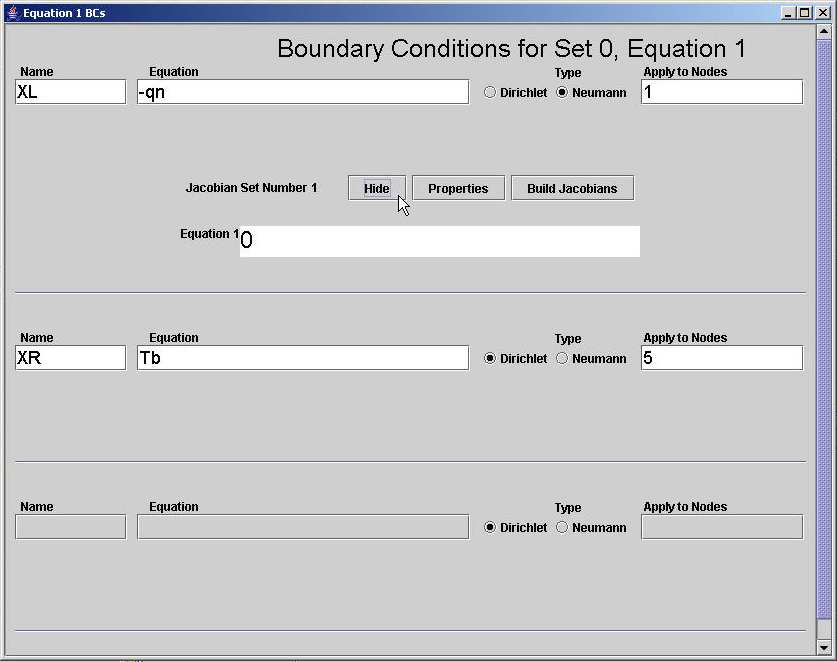
Figure 9. Boundary Condition parameters.

Submitting the job

1. As before, remember to configure the GUI, if it has not already been configured.
2. Navigate to the Submit panel.
3. For the Job Name, enter lab2.m
4. Use the File Chooser to select a Remote Working Directory on the remote machine.

a. Press the File Chooser button.
b. Select the file system view of the remote machine by pressing the Remote button.
c. Select a directory, like DATA1.
d. Press the open button. DATA1 should appear in the Input Data Directory field.

Figure 10. Selecting a remote directory.

5. Press the Submit button in the Submit panel.
6. Observe the results in the Status window.