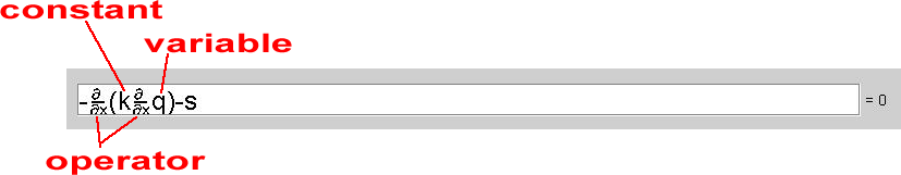
Figure 1. Equation term categorization.
Equation Builder
This documentation describes the components of the Equation Builder. For detail on HOW to build equations see the Tutorials.
Every equation term has 3 fundamental components: constants, operators, and variables (Figure 1). Every component that is put into an equation term MUST be defined before the equation is built. In some cases, a term may have zero constants, operators or variables. Constants are defined in either the Physical Parameters panel or the Iteration Parameters panel. Operators are predefined by the GUI and are shown in the toolbar at the top. Variables (dependent variables) can be English or Greek symbols and may have different characteristics applied to them as defined in the Variable Properties (see Help Topics Toolbar section for more information). Components to be used in an equation do not need to be defined in the toolbars at the top, but those toolbar buttons may be used to aid in building equations. Keyboard strokes may also be used to build equations. See the Tutorial for more detail.
Note: It is important to remember that the GUI does not perform mathematical calculations and it does not understand numbers. Once numbers are defined as symbols in the Physical Parameters table the symbols can be used in the equations.
Figure 1. Equation term categorization.
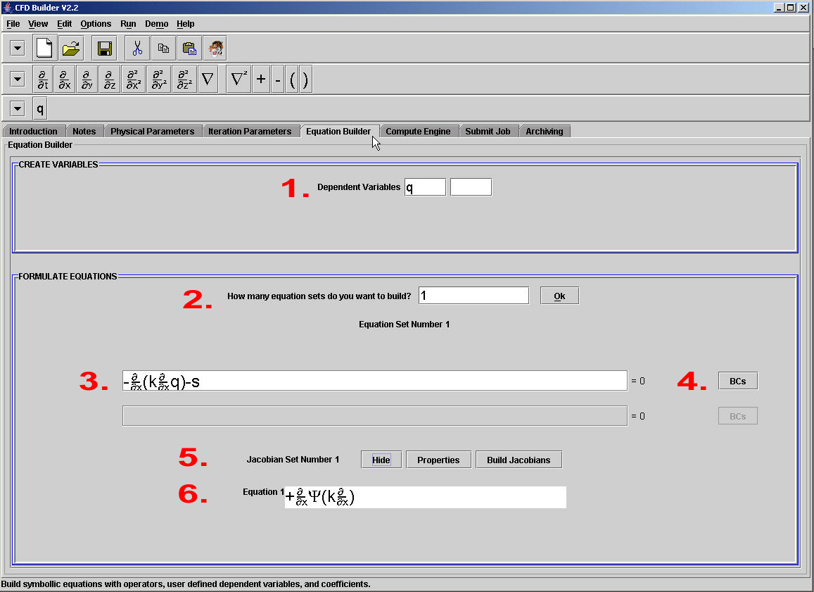
Figure 2. Equations Panel.
Figure 2 shows the Equations Panel with a simple example.
1. The dependent variables are defined for all equations and all equation sets. These dependent variables may be Greek or English letters and may have other characteristics defined in the Variable Properties.
2. The user must specify how many equation SETS will be built.There may be many equations in a single set, and there may be multiple sets. After entering the number of sets, press "Apply".
3. The equation is built in a text box by clicking on the text box and then entering information through keyboard strokes or using the toolbars at the top. See the Summary of Equation Building Rules for more information. To enter additional equations enter the next unoccupied box to activate it. NOTE: Be very careful not to enter any more equation boxes or sets than are absolutely necesary. At this time there is no way to deactivate a box that is active. Active equation boxes that contain no information may cause instabilities in the application.
4. All equations must have boundary conditions associated with them for well-posedness. No specification of a boundary condition implies a zero Neumann condition (nothing is done). To specify non-zero Neumann or a Dirichlet condition, press the BCs button.

Figure 3. Bounday Conditions Window for a single equation.
A boundary condition for eqach equation can be specified on any number of points, lines or surfaces.
a. The bounday must have a name. In a one-dimensional problem with the domain defined as a single line there are 2 boundaries, one on each end of the line. Here they are called XL and XR. A two-dimensional domain must have boundary names that correspond to the geometry file boundary names, as discussed in the Compute Engine Panel.
b. The value on the boundary is then specified. This may be an equation or a constant. Remember that this application sees all information symbollically. Here, qn and Tb are constants that were defined in the the Physical Parameters.
c. This application supports 2 types of boundary conditions: Dirichlet and Neumann.
d. The location of boundary must be specified. For 2-D and 3-D problems the boundaries are typically specified in a file, and the connection between the boundary values and the location is made through the boundary name. For simple 1-D problems, the user may specify the node number(s) of the boundary location.
e. Since Neumann boundaries are equations, they also contain Jacobians which may be specified here. A more detailed description of the Jacobians is given below. Note in this case that the Neumann condition specified a constant, thus the Jacobian is zero.
5. Every equation, whether linear or not, is treated as a non-linear equation. This is done for consistency and generality, since linear equations are a special case of non-linear equations. The way we choose to solve non-linear equations is through the Newton iterative method where Jacobians must be developed. By default, the Jacobians are hidden.
An automated Jacobian Building function is provided, but requires some information, specified in the Jacobian Propeties.
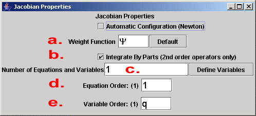
Figure 4. Jacobian Properties.
a. The Jacobian may be weighted by a function (or none if preferred). The default weight function is a capital PSI.
b. The weight function may be used for weak statement development, breaking down 2nd order operators into 1st order components.
c. The Jacobian must initially contain the same number of dependent variables as there are equations in the set. This is a requirement for the automated Jacobian Building process.
d. The Jacobians will be formed top-down from the equations. But the equation order need not be top-down.
e. Like the previous step, the Jacobian order need not be the same as the equation order. These two options should only effect visual appearance of the Jacobian.
The automated Jacobian Building tool is simplistic at best, and is only meant to get the user started on the general syntax and format of Jacobians. It is the user's responsibility to ensure that the Jacobians are correct before building script.
6. The Jacobians in a matrix format and can be edited by the user.