Tutorial 1

This tutorial allows the user to get comfortable with the graphical user interface (GUI) before actually building equations and running simulations. To supplement this tutorial, it is recommended that the user get familiar with the GUI architecture as described in the overview. To summarize the key points, the GUI is considered to consist of two distinct parts: equation interpretation, and the compute engine interface. Together these two pieces create a text file, or files, that can be used by a compute engine to solve a system of equations. The equation interpreter has few restrictions in how equations can be built, but the compute engine interface may have many. It is critical that the user understand the rules of building equations for the specific compute engine of choice.

At this time the user should have all requirements that are outlined in Getting Started. To start the GUI click here. A Java Web Start window will appear, and shortly afterward the GUI should open, showing the status of panels as they are loaded.

Terminology of this tutorial is introduced in Figure 1, and is fairly common among all related documentation. As seen below, the menu bar and toolbar are typical of most graphical applications. The tabs, also referred to as panels, are logical groupings of a computational simulation. Each panel will have some combination of labels, text boxes and buttons to guide the user through the creation of a simulation.

Figure 1. The GUI lingo.

Configuring the GUI

If running remotely, the GUI should always be configured first (this assumes a working network connection). Configuration of the GUI means that you are getting path and executable names for applications that will run on remote machines. The user does not need any knowledge of the remote machine, only a username and password. If the server recognizes the user (authenticates the user), the GUI will automatically provide the server configuration. These GUI configuration steps must be performed every time the GUI is started. However, once the GUI is started, the configuration is good for any number of simulations to be performed until the GUI is closed.

After completing the above steps, the GUI will start, showing the Configuration/Introduction Panel.
Enter your username and password, and appropriate server name with port number. Then press "Apply" (Figure 2).
If the server connection and user authentication is successful, the fields below the username and password boxes will show the remote machine configuration.

See Configuration Panel for more information.

Figure 2. Configuring the GUI.

Opening a demonstrantion

Next, go to the menu bar and under "Demo" select the Lab 2, 1-D Heat Conduction problem (Figure 2).

Figure 2. Selecting the 1-D Heat Conduction example.

A brief discussion about the contents of this example (browsing panels from left to right).

Notes - Notes are provided describing the variable names used in this example. The energy norm and mesh convergence information is data that can be added to the GUI generated script.

Physical Parameters - All physical parameters associated with this equation are defined in the Physical Parameter tables. Notice that the source term is defined as "nodal". This means that there is a value for the conductivity at every node point, and in this case it is the same for every point. For a simple 1-D problem the domain (X1) can be defined in the in the Physical Parameters, but for a more complicated geometry the domain is defined in a separate file. There are several parameters defined, but not all are used in the equations. Items in the boundary conditions maybe defined here as well.

Iteration Parameters - This is a linear and steady state equation so no integration or iteration parameters are required.

Equation Builder - The system of equations in this demonstration contains one equation set, with one equation, and two terms. The first term is the diffusion term of the energy equation with two derivatives in the x-direction, and second is a source term. The state variable, q, is the only dependent variable and represents the temperature. The conductivity, k, is defined in the Physical Parameters as a global constant, but could be a nodal constant varying with x. Boundary Conditions - On the left node (node 1, called XL) a constant Neumann boundary condition is applied (qn). On the right node (node 5, called XR), the boundary is maintained at a constant temperature, Tb. Values for Tb and qn are defined in the Physical Parameters.

Compute Engine - The default Matlab solver will be used, and the 1-D domain is defined in the Physical Parameters. No data input is required in the Compute Engine Panel.

Submit Job - This simulation will be called lab2.m and will be stored on a remote machine in the users directory called DATA1.

Archiving - Archiving is provided for advanced users and will not be discussed here.

Executing a job

Click on the "Submit Job" tab. This panel, Figure 3, is the connection between the GUI and the compute engine.

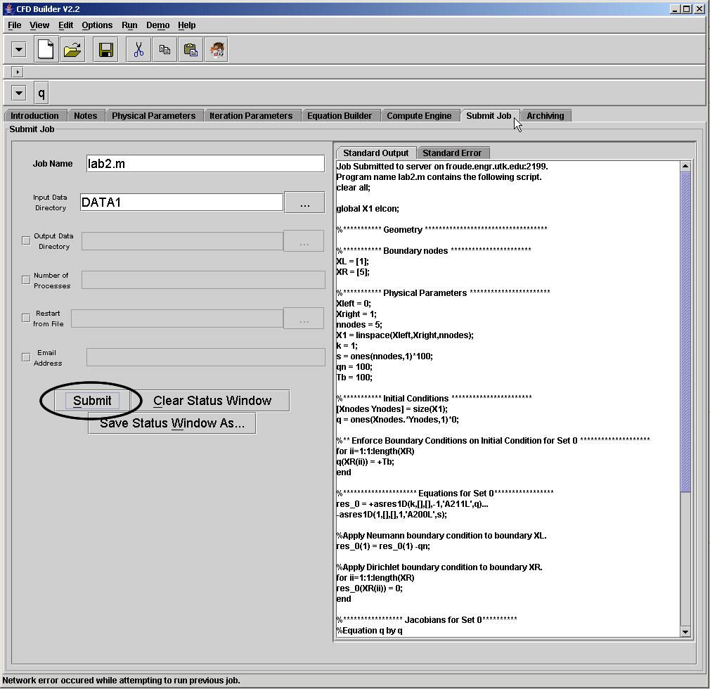
Figure 3. Submit Job Panel.

Press the Submit button. The GUI generated script should appear in the Status window so that the user may verify that the correct script was sent to the compute engine. After a short pause, results of the simulation should appear at the botton of the Status window. The user may need to scroll down to see the results. Tip: watch the scroll bar to the right for changes. This will help identify when new information has come into the Status window. Notice that there are 5 nodes in the domain, and 5 results are returned, one for each node.

As the user studies more complicated problems it is easy to lose track of whether a problem is due to the client application, the compute engine toolbox, the network, or the input data. When troubles occur, one way to check the status of the network, and to some degree the GUI, is to re-run this demonstration as it should always work.