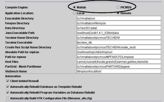
Figure 1. Ensure that the Matlab option is selected.
Matlab Specifics
Introduction/Configuration
Ensure that the Matlab option is selected, especially after authentication to a remote machine.
Figure 1. Ensure that the Matlab option is selected.
Physical Parameters
There are 3 Matlab specific notes to be made in the Physical Parameters Panel.
1. If a geometry file is not specified in the Compute Engine Panel, then the geometry MUST be specified in the Physical Parameter table. Variables for the dimensions x,y, and z are X1, X2, and X3. The variables are expected and must be specified. Since a 1-D domain is simply a line, Matlab script is used to define the line, as described next.
2. The third column is "literal" variable data. That is, this can be Matlab specific text which might typically appear on the right-hand side of an equation in a Matlab file. In the example of Figure 2, the domain is a line made of points starting at Xleft, ending at Xright, and comprised of nnodes number of points. Row 4 in this figure will show up in the Matlab script as X1=linspace(Xleft,Xright,nnodes);
3. The last column tells the GUI what kind of data it is dealing with (remember
that all information in the GUI is symbollic. The GUI does not understand Matlab
script, only symbols. So the data type must be supplied). The data types are
global (constant over the entire domain), element averaged, or applied to the
nodes in the domain. Matlab compute engine errors occur due to an incorrect
data type specification more often than any other cause. Note that the domain
(X1) is nodal data, but is not specified as nodal. Only information that is
used in an equation, Jacobian, or boundary condition, needs to have a data type
defined. In this example, X1 is not used in any of those three areas, so defining
it as nodal is not necessary.

Figure 2. Physical Parameters Panel.
Iteration/Integration Parameters
Unsteady problems require time variables for the time integration loop. These variables must be supplied to the Matlab Interface with names as shown, but not necessarily in this order..
a. delta_t - time step increment
b. theta - integration impliciness factor
c. start - step start number
d. inc - time step increment value
e. stop - time step stop number
When translated to Matlab script this will look like,
for timeLoop=start : inc : stop
...
delta_q = (M_0+theta*delta_t*jac_0)\(-delta_t*res_0);
...
end
In the example of Figure 3 the time stepping is done as the number of steps (i.e. for step=1:1:50), but the user could also supply delta_t information and increment the loop over time, like,
time_start = 0.0;
time_stop=100.0;
start=time_start;
inc=delta_t;
stop=time_stop;
for timeLoop=start : inc : stop
...

Figure 3. Unsteady loop variables for time integration.
Non-linear equations will iterate in a for loop to some convergence criteria. The following variable names must be supplied to the Matlab Interface:
a. in_maxit - the maximum iterations that are allowed by the for loop. It is important that the user check solution results to ensure that the problem converged with the maximum iteration criteria.
b. in_eps - (or inner loop epsilon) the solution convergence criteria
For simulations with multiple sets of equations the variables out_maxit, and out_eps may be used for one outer for loop around all sets of equations, rather than an inner for loop around each equation set.
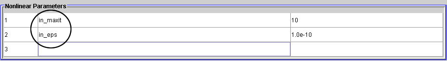
Figure 4. Non-linear loop variables for non-linear iteration.
At this time the Matlab Interface can solve problems that are:
a. linear and steady
b. nonlinear and steady
c. linear and unsteady
but non-linear and unsteady examples have not been developed.
Equation Builder
The Matlab Interface expects the Jacobians to have a weight function. The GUI default (capital PSI) is sufficient.
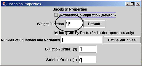
Figure 5. The jacobian weight function.
If a Matlab geometry file is specified in the Compute Engine Panel, then the boundary condition names must coincide with the boundary names in the file, as discussed in the Compute Engine Panel, and Equation Panel Help Topics.
Compute Engine
Matlab specific details in the Compute Engine Panel has been discussed in the Compute Engine Panel Help Topics.
Submit Job
The Matlab Interface generates serial code and has no need for restart file information. Also, the simple academic problems that the Matlab Interface creates are small enough that they run fairly quickly. Thus, the first two text boxes are the only ones required to run Matlab.
NOTE: When the GUI executes the Matlab script that it generated, it gives the script a Job Name. For Matlab, this name MUST be suffixed by ".m", as shown in Figure 6.
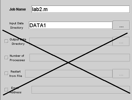
Figure 6. Matlab data management options.
Options
The Matlab Interace generates script equations from user specified input based on predefined element bases. The degree of the basis is understood by a suffix on the end of the basis name defining the degree. For example,
a. A200L - linear
b. A200Q - quadratic
c. A200C - cubic
d. A200H - Hermite
The Matlab finite element tools are found in a toolbox which contains residual and Jacobian assembly functions (asres and asjac), and the element libraries. The GUI will allow the user to choose any element matrix of any degree desired, but that does not mean that the element matrix is in the library.
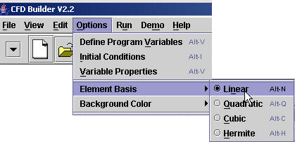
Figure 7. Element basis options.
As of December 2003, the following element matrices cans be found in the element library,
A200H A201Q A211L A3000Q A3011C A3101L B200L B211L B222L
A200L A210L A211Q A3001L A3011L A3101Q B201L B212L B3001L
A200Q A210Q A222H A3001Q A3011Q A3110L B202L B220L B3002L
A201L A211C A3000L A3010L A3100L A3110Q B210L B221L
Demo
The first six demonstrations are Matlab examples.
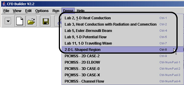
Figure 8. Matlab demonstrations.
Running Matlab locally
The GUI generates Matlab script that the user may save to the local hard drive. If Matlab is on the local machine, Matlab will run that saved script provided the user has the fempse toolbox (a directory of Matlab files) installed on the local hard drive, and the user has supplied the path name of the toolbox to fempse.
1. Download the fempse toolbox from here.
2. Unzip the fempse file. A directory will be created (called fempse) that will contain all the required Matlab files.
3. Open Matlab.
4. Go to File -> set Path -> add Folder
5. Browse the file directories and select the fempse folder you unzipped.
6. "Save" the configuration.
The GUI generated files can now be run from within Matlab.